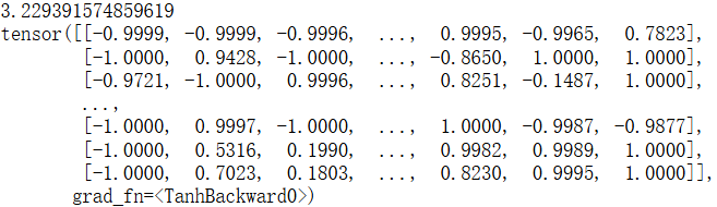
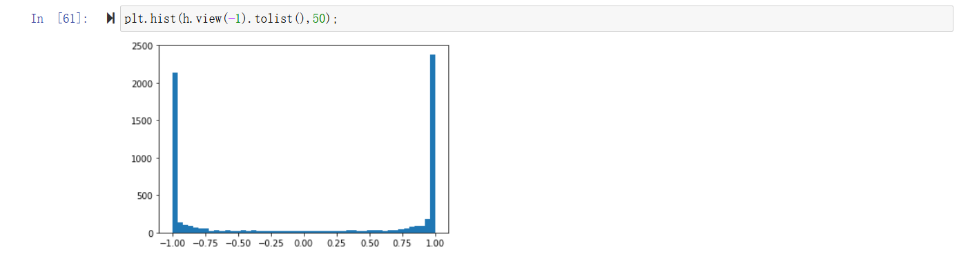
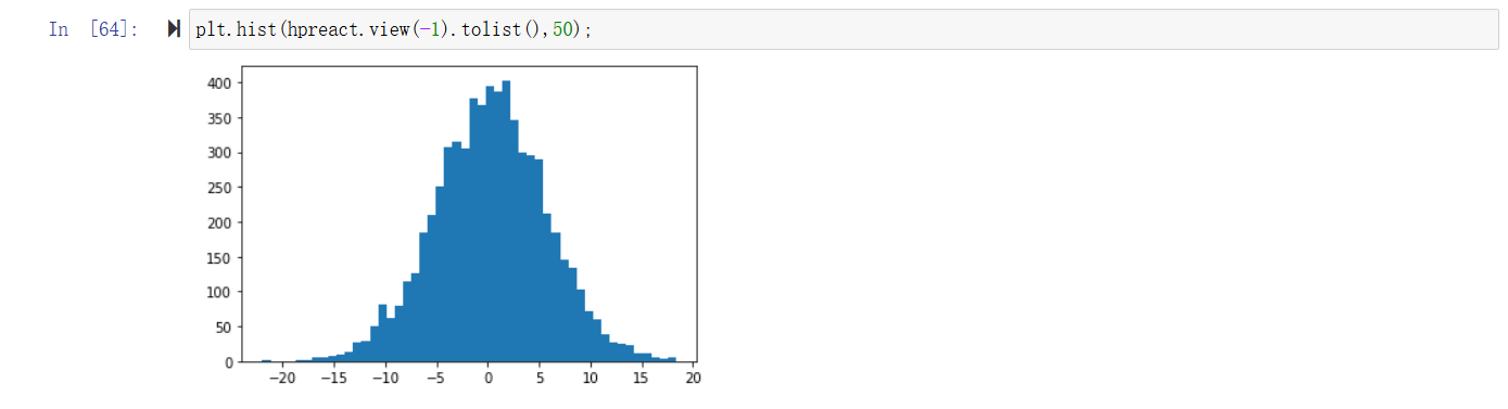
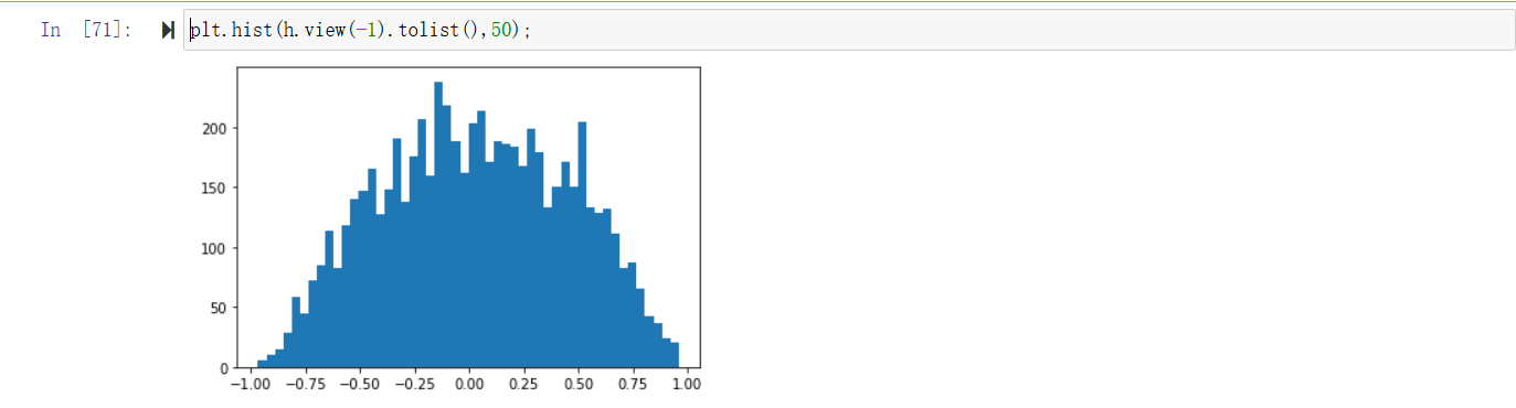
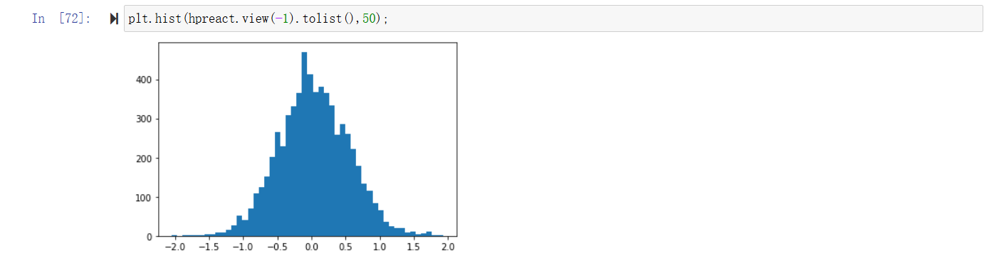
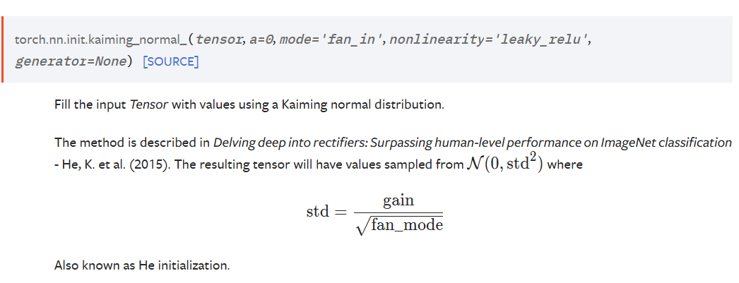
可以看到确实hpreact的分布很广,这导致了h值大部分为-1和1,而y = tanh(x), grad x = (1-tanh(x)^2)*grad y, 由于tanh(x)的值偏向于1和-1,导致grad y无法传递到x上,同样无法反向传播到前面的参数上,导致很多步的优化都无法大幅改变参数(无效的改变)。直接的,我们期待hpreact的值减小,所以修改参数w1和b1
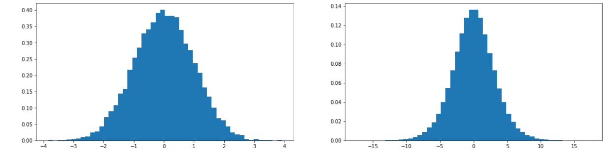
x = torch.randn(1000,10) w = torch.randn(10,200) y = x @ w print(x.mean(), x.std()) print(y.mean(), y.std()) plt.figure(figsize=(20,5)) plt.subplot(121) plt.hist(x.view(-1).tolist(),50,density=True) plt.subplot(122) plt.hist(y.view(-1).tolist(),50,density=True)
x = torch.randn(1000,10) w = torch.randn(10,200) / (10**0.5) # 这里说的fin就是第一个维度,10 y = x @ w print(x.mean(), x.std()) print(y.mean(), y.std()) plt.figure(figsize=(20,5)) plt.subplot(121) plt.hist(x.view(-1).tolist(),50,density=True) plt.subplot(122) plt.hist(y.view(-1).tolist(),50,density=True)
with torch.no_grad(): # pass the training set through emb = C[Xtr] embcat = emb.view(emb.shape[0], -1) hpreact = embcat @ W1 # + b1 # measure the mean/std over the entire training set bnmean = hpreact.mean(0, keepdim=True) bnstd = hpreact.std(0, keepdim=True)
# MLP revisited n_embd = 10# the dimensionality of the character embedding vectors n_hidden = 200# the number of neurons in the hidden layer of the MLP
parameters = [C, W1, W2, b2, bngain, bnbias] print(sum(p.nelement() for p in parameters)) # number of parameters in total for p in parameters: p.requires_grad = True
# build the dataset block_size = 3# context length: how many characters do we take to predict the next one?
defbuild_dataset(words): X, Y = [], [] for w in words: context = [0] * block_size for ch in w + '.': ix = stoi[ch] X.append(context) Y.append(ix) context = context[1:] + [ix] # crop and append
X = torch.tensor(X) Y = torch.tensor(Y) print(X.shape, Y.shape) return X, Y
import random random.seed(42) random.shuffle(words) n1 = int(0.8*len(words)) n2 = int(0.9*len(words))
# MLP revisited n_embd = 10# the dimensionality of the character embedding vectors n_hidden = 200# the number of neurons in the hidden layer of the MLP
parameters = [C, W1, W2, b2, bngain, bnbias] print(sum(p.nelement() for p in parameters)) # number of parameters in total for p in parameters: p.requires_grad = True
with torch.no_grad(): # pass the training set through emb = C[Xtr] embcat = emb.view(emb.shape[0], -1) hpreact = embcat @ W1 # + b1 # measure the mean/std over the entire training set bnmean = hpreact.mean(0, keepdim=True) bnstd = hpreact.std(0, keepdim=True)
n_embd = 10# the dimensionality of the character embedding vectors n_hidden = 100# the number of neurons in the hidden layer of the MLP g = torch.Generator().manual_seed(2147483647) # for reproducibility
# 下面对参数进行了进一步的调整 with torch.no_grad(): # last layer: make less confident layers[-1].gamma *= 0.1 #layers[-1].weight *= 0.1 # all other layers: apply gain for layer in layers[:-1]: ifisinstance(layer, Linear): layer.weight *= 1.0#5/3
parameters = [C] + [p for layer in layers for p in layer.parameters()] print(sum(p.nelement() for p in parameters)) # number of parameters in total for p in parameters: p.requires_grad = True
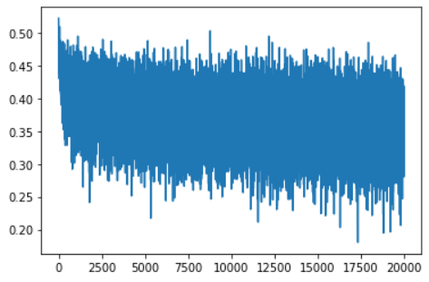
# same optimization as last time max_steps = 200000 batch_size = 32 lossi = [] ud = []
for i inrange(max_steps): # minibatch construct ix = torch.randint(0, Xtr.shape[0], (batch_size,), generator=g) Xb, Yb = Xtr[ix], Ytr[ix] # batch X,Y # forward pass emb = C[Xb] # embed the characters into vectors x = emb.view(emb.shape[0], -1) # concatenate the vectors for layer in layers: x = layer(x) loss = F.cross_entropy(x, Yb) # loss function # backward pass for layer in layers: #强制PyTorch保留神经网络各层输出的梯度信息,即使这些输出是中间计算过程(非叶子节点)。为了后面的可视化 layer.out.retain_grad() # AFTER_DEBUG: would take out retain_graph for p in parameters: p.grad = None loss.backward() # update lr = 0.1if i < 150000else0.01# step learning rate decay for p in parameters: p.data += -lr * p.grad
# track stats if i % 10000 == 0: # print every once in a while print(f'{i:7d}/{max_steps:7d}: {loss.item():.4f}') lossi.append(loss.log10().item()) with torch.no_grad(): ud.append([((lr*p.grad).std() / p.data.std()).log10().item() for p in parameters])
if i >= 1000: break# AFTER_DEBUG: would take out obviously to run full optimization
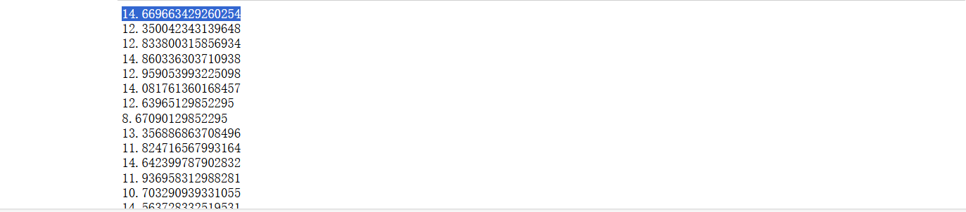
0/ 200000: 3.2870
下面是通过可视化来诊断训练过程,一些诊断方法
1 2 3 4 5 6 7 8 9 10 11 12
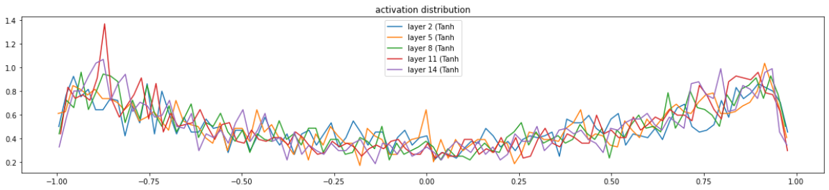
# visualize histograms plt.figure(figsize=(20, 4)) # width and height of the plot legends = [] for i, layer inenumerate(layers[:-1]): # note: exclude the output layer ifisinstance(layer, Tanh): # 这里只对tanh进行可视化,因为比较方便可视化 t = layer.out print('layer %d (%10s): mean %+.2f, std %.2f, saturated: %.2f%%' % (i, layer.__class__.__name__, t.mean(), t.std(), (t.abs() > 0.97).float().mean()*100)) # 网络输出的均值,方差,饱和度(绝对值超过0.97的占比) hy, hx = torch.histogram(t, density=True) # 这个函数绘制直方图,density=True是按照概率密度来计算的,这里的概率密度和概率不一样,和区间长度也有关,所以会大于1,频数/(总量*区间长度) plt.plot(hx[:-1].detach(), hy.detach()) legends.append(f'layer {i} ({layer.__class__.__name__}') plt.legend(legends); plt.title('activation distribution')
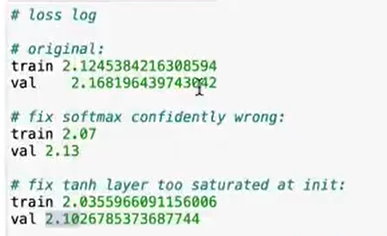
下面是输出结果,可以看到mean大致为0,std还不错,saturated比较小,tanh比较合理
layer 2 ( Tanh): mean -0.00, std 0.63, saturated: 2.78%
layer 5 ( Tanh): mean +0.00, std 0.64, saturated: 2.56%
layer 8 ( Tanh): mean -0.00, std 0.65, saturated: 2.25%
layer 11 ( Tanh): mean +0.00, std 0.65, saturated: 1.69%
layer 14 ( Tanh): mean +0.00, std 0.65, saturated: 1.88%
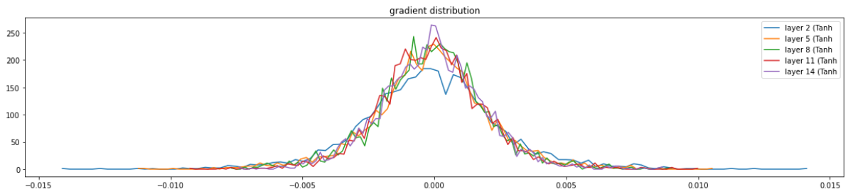
上面是对value进行了可视化,下面对grad进行可视化
1 2 3 4 5 6 7 8 9 10 11 12
# visualize histograms plt.figure(figsize=(20, 4)) # width and height of the plot legends = [] for i, layer inenumerate(layers[:-1]): # note: exclude the output layer ifisinstance(layer, Tanh): t = layer.out.grad print('layer %d (%10s): mean %+f, std %e' % (i, layer.__class__.__name__, t.mean(), t.std())) hy, hx = torch.histogram(t, density=True) plt.plot(hx[:-1].detach(), hy.detach()) legends.append(f'layer {i} ({layer.__class__.__name__}') plt.legend(legends); plt.title('gradient distribution')
layer 2 ( Tanh): mean -0.000000, std 2.640702e-03
layer 5 ( Tanh): mean +0.000000, std 2.245584e-03
layer 8 ( Tanh): mean -0.000000, std 2.045742e-03
layer 11 ( Tanh): mean +0.000000, std 1.983134e-03
layer 14 ( Tanh): mean -0.000000, std 1.952382e-03
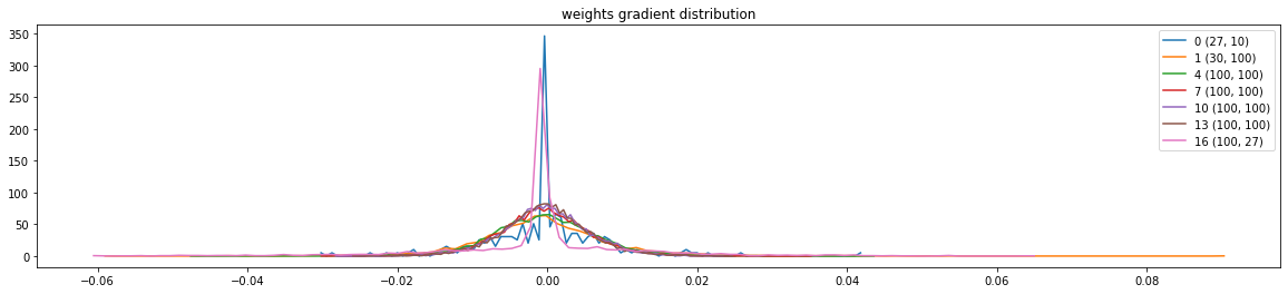
下面对grad/value进行了测试,这个值其实意义不是很明显
1 2 3 4 5 6 7 8 9 10 11 12
# visualize histograms plt.figure(figsize=(20, 4)) # width and height of the plot legends = [] for i,p inenumerate(parameters): t = p.grad if p.ndim == 2: print('weight %10s | mean %+f | std %e | grad:data ratio %e' % (tuple(p.shape), t.mean(), t.std(), t.std() / p.std())) hy, hx = torch.histogram(t, density=True) plt.plot(hx[:-1].detach(), hy.detach()) legends.append(f'{i}{tuple(p.shape)}') plt.legend(legends) plt.title('weights gradient distribution');
weight (27, 10) | mean +0.000000 | std 8.020534e-03 | grad:data ratio 8.012630e-03
weight (30, 100) | mean +0.000246 | std 9.241077e-03 | grad:data ratio 4.881091e-02
weight (100, 100) | mean +0.000113 | std 7.132879e-03 | grad:data ratio 6.964619e-02
weight (100, 100) | mean -0.000086 | std 6.234305e-03 | grad:data ratio 6.073741e-02
weight (100, 100) | mean +0.000052 | std 5.742187e-03 | grad:data ratio 5.631483e-02
weight (100, 100) | mean +0.000032 | std 5.672205e-03 | grad:data ratio 5.570125e-02
weight (100, 27) | mean -0.000082 | std 1.209416e-02 | grad:data ratio 1.160106e-01
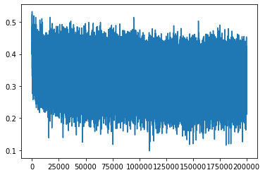
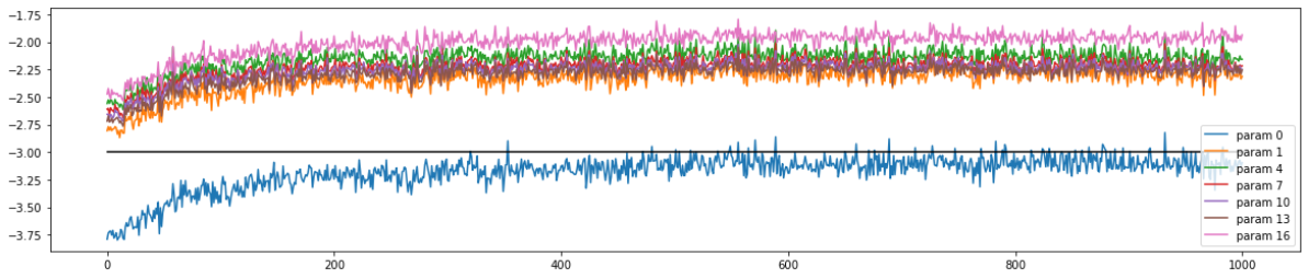
plt.figure(figsize=(20, 4)) legends = [] for i,p inenumerate(parameters): if p.ndim == 2: plt.plot([ud[j][i] for j inrange(len(ud))]) legends.append('param %d' % i) plt.plot([0, len(ud)], [-3, -3], 'k') # these ratios should be ~1e-3, indicate on plot plt.legend(legends);
1 2 3 4 5 6 7 8 9 10 11 12 13 14 15 16 17 18 19
@torch.no_grad() # this decorator disables gradient tracking defsplit_loss(split): x,y = { 'train': (Xtr, Ytr), 'val': (Xdev, Ydev), 'test': (Xte, Yte), }[split] emb = C[x] # (N, block_size, n_embd) x = emb.view(emb.shape[0], -1) # concat into (N, block_size * n_embd) for layer in layers: x = layer(x) loss = F.cross_entropy(x, y) print(split, loss.item())
# put layers into eval mode for layer in layers: layer.training = False split_loss('train') split_loss('val')
# sample from the model g = torch.Generator().manual_seed(2147483647 + 10)
for _ inrange(20): out = [] context = [0] * block_size # initialize with all ... whileTrue: # forward pass the neural net emb = C[torch.tensor([context])] # (1,block_size,n_embd) x = emb.view(emb.shape[0], -1) # concatenate the vectors for layer in layers: x = layer(x) logits = x probs = F.softmax(logits, dim=1) # sample from the distribution ix = torch.multinomial(probs, num_samples=1, generator=g).item() # shift the context window and track the samples context = context[1:] + [ix] out.append(ix) # if we sample the special '.' token, break if ix == 0: break print(''.join(itos[i] for i in out)) # decode and print the generated word