1
2
3
4
5
6
7
8
9
10
11
12
13
14
15
16
17
18
19
20
21
22
23
24
25
26
27
28
29
30
31
32
33
34
35
36
37
38
39
40
41
42
43
44
45
46
47
48
49
50
51
52
53
54
55
56
57
58
59
60
61
62
63
64
65
66
67
68
69
70
71
72
73
74
75
76
77
78
79
80
81
82
83
84
85
86
87
88
89
90
91
92
93
94
95
96
97
98
99
100
101
102
103
104
105
106
107
108
109
110
111
112
113
114
115
116
117
118
119
120
121
122
123
124
125
126
127
128
129
130
131
132
133
134
135
136
137
138
139
140
141
142
143
144
145
146
147
148
149
150
151
152
153
154
155
156
157
158
159
160
161
162
163
164
165
| import torch
import matplotlib.pyplot as plt
import torch.nn.functional as F
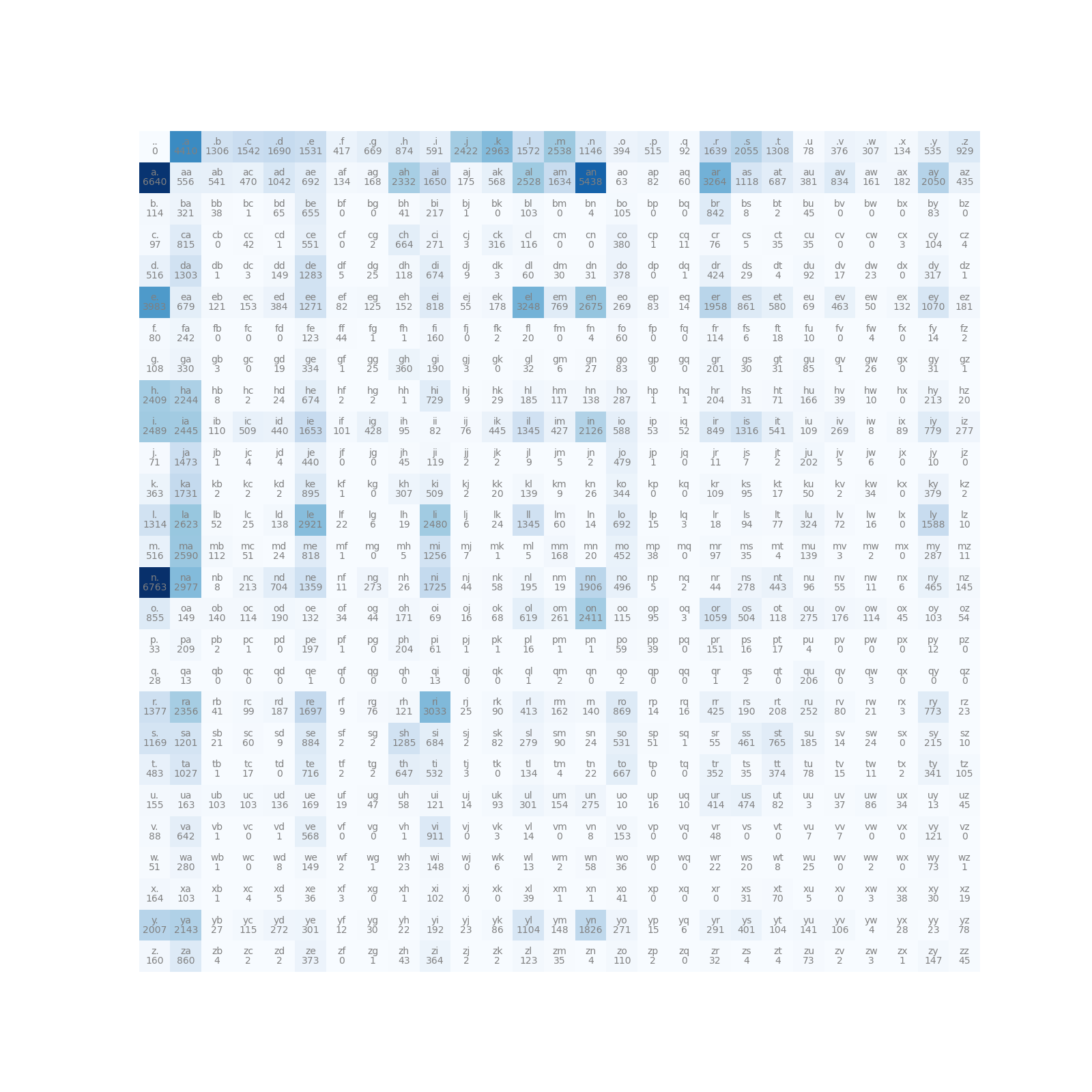
N = torch.zeros((27,27),dtype=torch.int32)
words = open("names.txt", "r").read().splitlines()
chars = sorted(list(set("".join(words))))
stoi = {s:i+1 for i,s in enumerate(chars)}
stoi['.'] = 0
itos = {i:s for s,i in stoi.items()}
for w in words:
chs = ['.'] + list(w) + ['.']
for ch1,ch2 in zip(chs, chs[1:]):
N[stoi[ch1],stoi[ch2]] += 1
plt.figure(figsize=(16,16))
plt.imshow(N, cmap='Blues')
for i in range(27):
for j in range(27):
chstr = itos[i] + itos[j]
plt.text(j, i, chstr, ha="center", va="bottom", color='gray')
plt.text(j, i, N[i, j].item(), ha="center", va="top", color='gray')
plt.axis('off')
P = (N+1).float()
P /= P.sum(1, keepdim=True)
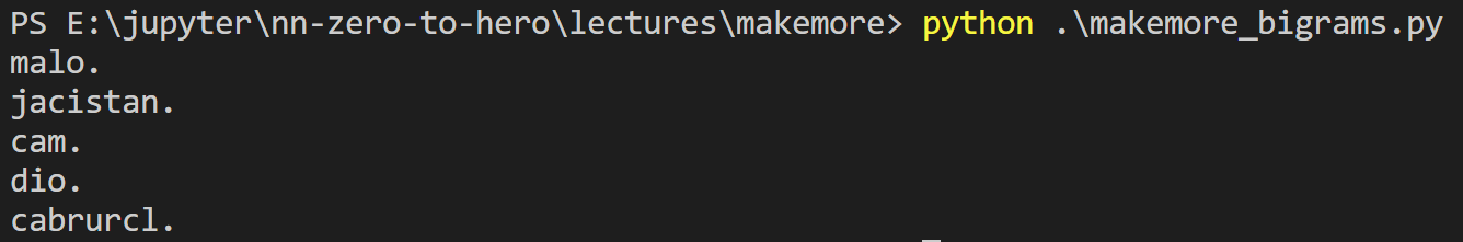
for i in range(5):
out = []
ix = 0
while True:
p = P[ix]
ix = torch.multinomial(p, num_samples=1, replacement=True).item()
out.append(itos[ix])
if ix == 0:
break
print(''.join(out))
log_likelihood = 0.0
n = 0
for w in words:
chs = ['.'] + list(w) + ['.']
for ch1,ch2 in zip(chs, chs[1:]):
p = P[stoi[ch1], stoi[ch2]]
log_likelihood += torch.log(p)
n += 1
print(f'{log_likelihood=}')
nll = -log_likelihood
print(f'{nll=}')
print(f'{nll/n}')
print('========================================')
xs, ys = [], []
for w in words[:1]:
chs = ['.'] + list(w) + ['.']
for ch1, ch2 in zip(chs, chs[1:]):
ix1 = stoi[ch1]
ix2 = stoi[ch2]
print(ch1, ch2)
xs.append(ix1)
ys.append(ix2)
xs = torch.tensor(xs)
ys = torch.tensor(ys)
W = torch.randn((27, 27))
xenc = F.one_hot(xs, num_classes=27).float()
logist = xenc @ W
counts = torch.exp(logist)
probs = counts / counts.sum(1, keepdim=True)
print(probs.shape)
nlls = torch.zeros(5)
for i in range(5):
x = xs[i].item()
y = ys[i].item()
print('--------')
print(f'bigram example {i+1}: {itos[x]}{itos[y]} (indexes {x},{y})')
print('input to the neural net:', x)
print('output probabilities from the neural net:', probs[i])
print('label (actual next character):', y)
p = probs[i, y]
print('probability assigned by the net to the the correct character:', p.item())
logp = torch.log(p)
print('log likelihood:', logp.item())
nll = -logp
print('negative log likelihood:', nll.item())
nlls[i] = nll
print('=========')
print('average negative log likelihood, i.e. loss =', nlls.mean().item())
print('==================')
xs, ys = [], []
for w in words:
chs = ['.'] + list(w) + ['.']
for ch1, ch2 in zip(chs, chs[1:]):
ix1 = stoi[ch1]
ix2 = stoi[ch2]
xs.append(ix1)
ys.append(ix2)
xs = torch.tensor(xs)
ys = torch.tensor(ys)
num = xs.nelement()
print('number of examples: ', num)
W = torch.randn((27, 27), requires_grad=True)
for k in range(1000):
xenc = F.one_hot(xs, num_classes=27).float()
logits = xenc @ W
counts = logits.exp()
probs = counts / counts.sum(1, keepdims=True)
loss = -probs[torch.arange(num), ys].log().mean() + 0.01*(W**2).mean()
print(loss.item())
W.grad = None
loss.backward()
W.data += -50 * W.grad
for i in range(5):
out = []
ix = 0
while True:
xenc = F.one_hot(torch.tensor([ix]), num_classes=27).float()
logits = xenc @ W
counts = logits.exp()
p = counts / counts.sum(1, keepdims=True)
ix = torch.multinomial(p, num_samples=1, replacement=True).item()
out.append(itos[ix])
if ix == 0:
break
print(''.join(out))
|